Introduction
Time series forecasting models are analytical tools that predict future values based on historical data points ordered chronologically. These models are crucial in various fields, such as finance, economics, weather forecasting, and business planning. Standard techniques include autoregressive integrated moving average (ARIMA), exponential smoothing methods like Holt-Winters, and machine learning algorithms such as neural networks and support vector machines. Time series forecasting involves identifying patterns, trends, and seasonal fluctuations within the data to generate accurate predictions, aiding decision-making processes and strategic planning for businesses and organizations.
Table of Content
- Introduction
- Types of Time Series Forecasting Models
- Advanced Techniques for Time Series Forecasting
- Case Studies and Applications
Types of Time Series Forecasting Models
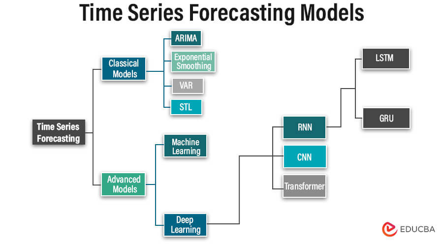
1. Classical Models:
- Autoregressive Integrated Moving Average (ARIMA):
ARIMA models represent traditional linear models utilized for capturing temporal dependencies within time series data, comprising three core components: autoregression (AR), differencing (I), and moving average (MA). These models are efficient for stationary data with identifiable or predictable patterns.
- Models of Exponential Smoothing:
Models of exponential smoothing, including Simple Exponential Smoothing (SES), Double Exponential Smoothing (Holt’s method), and Triple Exponential Smoothing (Holt-Winters method), represent straightforward yet potent methods for predicting time series data. These models allocate diminishing weights to previous observations exponentially, placing varying degrees of importance on recent versus older data points.
- Vector Autoregression (VAR):
Vector Autoregression (VAR) models build upon autoregressive models to analyze multivariate time series data. These models portray the connections between multiple variables by representing each variable as a linear function of its lagged values and those of other variables. VAR models prove valuable in examining interdependencies and generating combined forecasts for multiple time series.
- Seasonal Time Series Decomposition (STL):
STL is a method employed to break down a time series into its seasonal, trend, and residual elements. This breakdown empowers analysts to gain a deeper understanding of the inherent patterns within the data and can enhance forecasting precision.
2. Advanced Models:
- Machine Learning
Time series data can be effectively analyzed for forecasting and anomaly detection using various machine learning algorithms, encompassing decision trees, random forests, support vector machines, and neural networks. These algorithms exhibit the capacity to discern intricate patterns and correlations within the data, and in specific scenarios, they have demonstrated superior performance compared to conventional statistical models.
- Deep Learning
Deep learning, a subset of machine learning, employs neural networks with multiple layers (DNNs) to automatically learn hierarchical features from raw data. These networks, termed “deep” due to their numerous hidden layers, excel in capturing complex patterns. Training involves optimizing parameters using labeled data and algorithms to minimize prediction errors. Deep learning finds applications in various fields, including time series forecasting, where architectures like LSTM networks and CNNs are prevalent. Challenges include resource-intensive computations, data requirements, and guarding against overfitting. Nonetheless, it revolutionizes domains by empowering models to learn intricate patterns directly from data.
- Recurrent Neural Networks (RNNs):
RNNs are engineered to process sequential data by maintaining a hidden state that captures temporal dependencies. Variants such as Long Short-Term Memory (LSTM) and Gated Recurrent Unit (GRU) are particularly adept at analyzing time series due to their capability to capture long-term dependencies and address vanishing gradient issues.
I- Long Short-Term Memory (LSTM) Networks:
Within the domain of sequential data modeling, Long Short-Term Memory (LSTM) networks, a variant of recurrent neural networks (RNN), excel. Tailored for capturing long-term dependencies within data, LSTMs find widespread application in tasks such as time series forecasting, anomaly detection, and sequence generation.
II- GRU (Gated Recurrent Unit):
It is a simplified RNN architecture akin to LSTM but addresses the vanishing gradient issue. It uses gating mechanisms for information control, enabling long-term dependency capture. With fewer parameters and computations than LSTM, GRU is efficient and more accessible to train. Its update and reset gates manage information flow, aiding stability in training and enhancing sequential data analysis.
- Convolutional Neural Networks (CNNs):
Predominantly utilized in image processing, CNNs can also be employed in handling time series data by treating the data as a one-dimensional image. CNNs can extract hierarchical features from time series data, rendering them valuable for classification and anomaly detection tasks.
- Transformer:
Originally designed for natural language processing tasks, the Transformer architecture has also been applied to time series forecasting by enabling parallel processing and capturing long-range dependencies effectively.
Advanced Techniques for Time Series Forecasting
Advanced methodologies for analyzing time series encompass diverse techniques that use state-of-the-art statistical and machine-learning approaches. The following are several commonly employed advanced techniques:
Probabilistic Models for Time Series:
- Gaussian Processes (GPs): GPs represent a versatile and robust framework for modeling time series data. They afford a probabilistic depiction of the data, enabling the estimation of uncertainty and systematically integrating prior knowledge.
- Bayesian Structural Time Series (BSTS) Models: BSTS models constitute Bayesian hierarchical models designed to disentangle time series data into trend, seasonality, and regression components. They are particularly valuable for tasks involving forecasting and causal inference.
Ensemble Methods:
- Ensemble Forecasting: Ensemble methods amalgamate predictions from multiple models to enhance predictive accuracy and resilience. Techniques such as bagging, boosting, and stacking can be utilized for time series forecasting by consolidating predictions from diverse models.
- Model Combination: Rather than amalgamating forecasts, model fusion techniques merge distinct elements of multiple models. This may involve combining feature representations learned by different models or integrating the outputs of models at various aggregation levels.
Anomaly Detection Techniques
- Unsupervised Anomaly Detection: Approaches such as autoencoders and one-class SVMs are suitable for detecting anomalies in time series data without needing labeled examples. These methods are designed to learn and recognize normal patterns within the data, thus enabling the identification of deviations as anomalies.
- Semi-supervised and Weakly Supervised Anomaly Detection: In situations where labeled anomaly data is limited, using semi-supervised and weakly supervised anomaly detection techniques becomes relevant. These methods use a small quantity of labeled anomaly data and a larger volume of unlabelled data to enhance anomaly detection accuracy.
Enhancing Time Series Analysis:
- Transfer Learning: Transfer learning methods utilize the knowledge acquired from a one-time series domain to improve performance in another domain, especially when labeled data is limited. This involves fine-tuning or adapting pre-trained models or representations from related tasks to suit the target domain.
- Domain Adaptation: Domain adaptation techniques strive to align the distributions of source and target time series domains, ultimately improving generalization performance. This process encompasses various approaches, such as adversarial training, domain-invariant feature learning, or domain-specific regularization.
Case Studies and Applications
1. Stock Market Forecasting Using Time Series Analysis with ARIMA Model on Tesla Stock Price
Introduction
In the fast-paced world of financial markets, accurate forecasting of stock prices is crucial for investors, traders, and financial analysts. Time series analysis, mainly using models like Autoregressive Integrated Moving Average (ARIMA), is a popular method for predicting stock prices based on historical data. In this case study, we will apply the ARIMA model to forecast the stock price of Tesla, Inc. (TSLA), a leading electric vehicle and clean energy company.
Objective
The primary objective of this case study is to demonstrate the application of the ARIMA model for forecasting Tesla’s stock price based on historical price data. We aim to predict future price movements by analyzing past trends and patterns, enabling investors to make informed decisions.
Data Collection
We obtained historical stock price data for Tesla (TSLA) from a reliable financial data source such as Yahoo Finance or Quandl. The dataset includes daily closing prices of Tesla stock over a specified period, typically spanning several years.
Data Preprocessing
Before applying the ARIMA model, we preprocess the data to ensure its suitability for time series analysis:
- Data Cleaning: Remove any missing values or outliers from the dataset.
- Data Transformation: Log transformation or differencing may be applied to stabilize variance or remove trends.
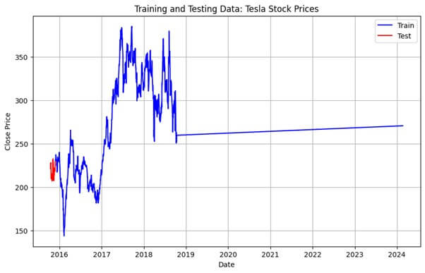
- Train-Test Split: Split the data into training and testing sets, typically using a 70-30 or 80-20 split.
Modeling
We fit an ARIMA model to the training data and tune the model parameters (p, d, q) based on the Akaike Information Criterion (AIC) or other suitable criteria. The ARIMA model consists of three main components:
- Autoregression (AR): The model captures the linear relationship between the current and lagged observations.
- Integration (I): Differencing is applied to make the time series stationary, removing trends or seasonality.
- Moving Average (MA): The model considers the error terms from previous forecasts to predict future values.
Model Evaluation
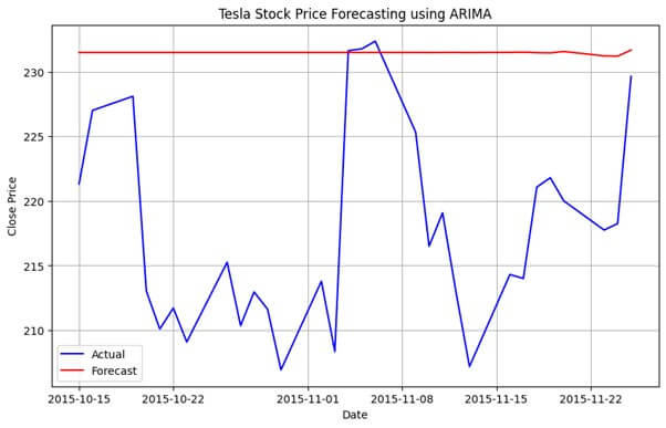
After training the ARIMA model, we evaluate its performance using the testing dataset. Common evaluation metrics for time series forecasting include Mean Absolute Error (MAE), Mean Squared Error (MSE), and Root Mean Squared Error (RMSE). Additionally, visual inspection of actual vs. predicted values and residual plots can provide insights into model accuracy and performance.
Forecasting
We generate forecasts for future Tesla stock prices using the trained ARIMA model. These forecasts represent the predicted closing prices over the forecast horizon, typically ranging from a few days to several weeks or months into the future.
Results and Conclusion
The final step involves analyzing the forecasting results and drawing conclusions about the performance of the ARIMA model in predicting Tesla stock prices. We assess the accuracy of the forecasts, identify any limitations or challenges encountered during the modeling process, and provide recommendations for future improvements or refinements.
Final Result
In this case study, we demonstrated the application of the ARIMA model for forecasting Tesla’s stock price based on historical data. Time series analysis with ARIMA provides a powerful framework for predicting stock prices and making informed investment decisions. By leveraging past trends and patterns, investors can gain valuable insights into future market movements, enabling them to optimize their investment strategies and achieve their financial objectives.
DataSet: (https://github.com/plotly/datasets/blob/master/tesla-stock-price.csv)
import pandas as pd
import numpy as np
import matplotlib.pyplot as plt
from statsmodels.tsa.arima.model import ARIMA
from sklearn.metrics import mean_squared_error
# Step 1: Data Preprocessing
data = pd.read_csv('tesla-stock-price.csv')
data['date'] = pd.to_datetime(data['date'])
data.set_index('date', inplace=True)# Step 2: Exploratory Data Analysis (EDA)
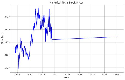
plt.figure(figsize=(10, 6))
plt.plot(data.index, data['close'], color='blue')
plt.title('Historical Tesla Stock Prices')
plt.xlabel('Date')
plt.ylabel('Close Price')
plt.grid(True)
plt.show()# Step 3: Model Development
train_data = data['close'][:-30] # Use data up to last 30 days for training
test_data = data['close'][-30:] # Use last 30 days for testing# Visualize Training and Testing Data on Single Graph
plt.figure(figsize=(10, 6))
plt.plot(train_data.index, train_data.values, color='blue', label='Train')
plt.plot(test_data.index, test_data.values, color='red', label='Test')
plt.title('Training and Testing Data: Tesla Stock Prices')
plt.xlabel('Date')
plt.ylabel('Close Price')
plt.legend()
plt.grid(True)
plt.show()# Fit ARIMA model
model = ARIMA(train_data, order=(5,1,0))
result = model.fit()
print(result.summary())# Step 4: Evaluation
predictions = result.forecast(steps=len(test_data))mse = mean_squared_error(test_data, predictions)
rmse = np.sqrt(mse)
print("Root Mean Squared Error (RMSE):", rmse)# Step 5: Forecasting
plt.figure(figsize=(10, 6))
plt.plot(data.index[-30:], test_data, color='blue', label='Actual')
plt.plot(data.index[-30:], predictions, color='red', label='Forecast')
plt.title('Tesla Stock Price Forecasting using ARIMA')
plt.xlabel('Date')
plt.ylabel('Close Price')
plt.legend()
plt.grid(True)
plt.show()2. Financial Time Series Analysis – Forecasting Real GDP
Introduction
In this case study, we’ll explore how to perform financial time series analysis using real Gross Domestic Product (GDP) data. We aim to forecast future GDP values using an Autoregressive Integrated Moving Average (ARIMA) model.
Background
We have access to a macroeconomic dataset containing quarterly observations of various economic indicators. Our analysis will focus on the ‘realgdp’ column, representing the real GDP values over time.
Objective
We aim to build an ARIMA model to forecast future real GDP values based on historical data.
Data Preparation
- We start by loading the macroeconomic dataset and converting the ‘year’ and ‘quarter’ columns to appropriate data types.
- We create a new ‘date’ column by combining ‘year’ and ‘quarter’ and set it as the index of the DataFrame.
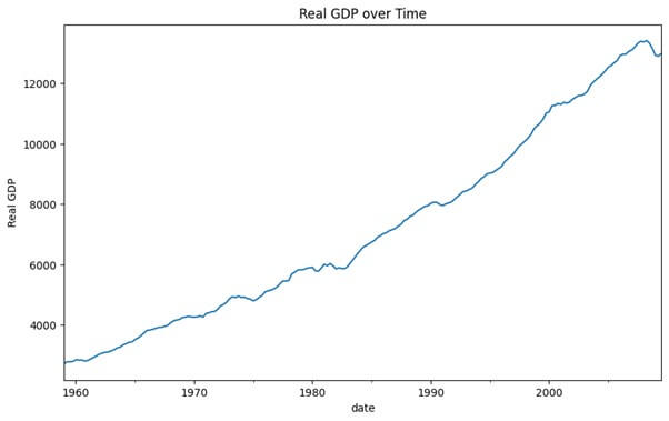
- To understand its trend and patterns, We visualize the real GDP data over time.
Modeling
- Given the characteristics of the real GDP data, we assume an ARIMA(1,1,1) model for demonstration purposes.
- We fit the ARIMA model to the real GDP data using the statsmodels library.
- After fitting the model, we print out the summary to analyze its performance and parameters.
Forecasting
- We forecast the next 10 periods (quarters) using the fitted ARIMA model.
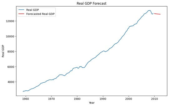
- We plot the real GDP values along with the forecasted values to visualize the predicted trend.
Final Result
Through this case study, we demonstrated the process of financial time series analysis and forecasting using an ARIMA model. By leveraging historical real GDP data and applying appropriate modeling techniques, we were able to generate forecasts for future GDP values. This analysis can provide valuable insights for policymakers, economists, and investors in making informed decisions.
pip install statsmodels
import numpy as np
import pandas as pd
import statsmodels.api as sm
import matplotlib.pyplot as plt
from statsmodels.tsa.arima.model import ARIMA
from sklearn.metrics import mean_squared_error

# Load the macroeconomic dataset
macrodata = sm.datasets.macrodata.load_pandas().data

# We'll use the 'realgdp' column for our time series analysis
macrodata['year'] = macrodata['year'].astype(int)
macrodata['quarter'] = macrodata['quarter'].astype(int)
macrodata['date'] = pd.to_datetime(macrodata['year'].astype(str) + 'Q' + macrodata['quarter'].astype(str))
macrodata.set_index('date', inplace=True)

# Plot the Real GDP data
macrodata['realgdp'].plot(title='Real GDP over Time', figsize=(10, 6))
plt.ylabel('Real GDP')
plt.show()
# Assuming an ARIMA(1,1,1) model for demonstration purposes
model = ARIMA(macrodata['realgdp'], order=(1, 1, 1))
model_fit = model.fit()
# Print out the summary
print(model_fit.summary())
# Forecast the next 10 periods
forecast = model_fit.forecast(steps=10)
# Plot the Real GDP and forecasted values
plt.figure(figsize=(10, 6))
plt.plot(macrodata.index, macrodata['realgdp'], label='Real GDP')
plt.plot(pd.date_range(macrodata.index[-1], periods=11, freq='Q')[1:], forecast, color='red', label='Forecasted Real GDP')
plt.title('Real GDP Forecast')
plt.xlabel('Year')
plt.ylabel('Real GDP')
plt.legend()
plt.show()Conclusion
Time series forecasting employs classical methods like ARIMA and exponential smoothing alongside advanced techniques such as machine learning and deep learning, including LSTM and CNN architectures. Probabilistic models and ensemble methods enhance accuracy, while anomaly detection techniques like autoencoders identify irregularities. Transfer learning and domain adaptation improve performance by leveraging related domain knowledge. Two case studies demonstrated time series analysis: forecasting Tesla’s stock prices with ARIMA and predicting real GDP values, emphasizing data preparation, model fitting, and projections. Accurate forecasting is pivotal for informed decision-making in finance and economics, offering valuable insights for investors, policymakers, and economists and aiding strategic planning processes.
Frequently Asked Questions (FAQs)
Q1: What are the main differences between classical and advanced time series forecasting models?
Answer: Classical models like ARIMA rely on traditional statistical techniques, while advanced models such as LSTM and CNN utilize machine learning and deep learning to capture complex patterns.
Q2: How do probabilistic models differ from deterministic forecasting methods?
Answer: Probabilistic models like Gaussian Processes provide a distribution of possible outcomes, accounting for uncertainty, whereas deterministic methods offer point estimates without considering uncertainty.
Q3: What are the primary challenges of applying deep learning models like LSTM and CNN to time series forecasting?
Answer: Challenges include data requirements for large-scale training, computational complexity, and guarding against overfitting due to the model’s susceptibility to noisy or limited data.
Recommended Articles
We hope that this EDUCBA information on “Time Series Forecasting Models” was beneficial to you. You can view EDUCBA’s recommended articles for more information.
