VBA Number Format

Updated April 8, 2023

Excel VBA Number Format

VBA Number Format though looks simple but it is very important to master them. In VBA, we have several ways to format numbers, we have the Number Format Function.

When it comes to range object, we use the property Range.NumberFormat to format numbers in the range. In today’s article, we will see how to use number format in range object to apply formatting style to our numbers.

What does Number Format Function do in VBA?

Just to remind you, excel stores all numerical values as serial numbers, be it date or time this will also be stored as serial numbers. According to the format given by the user to the serial number, it will display the result.

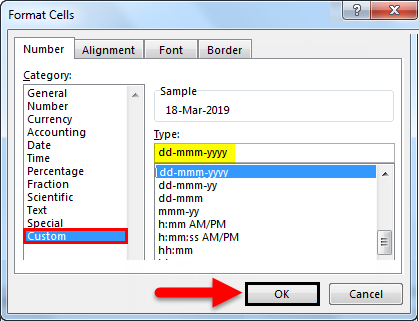
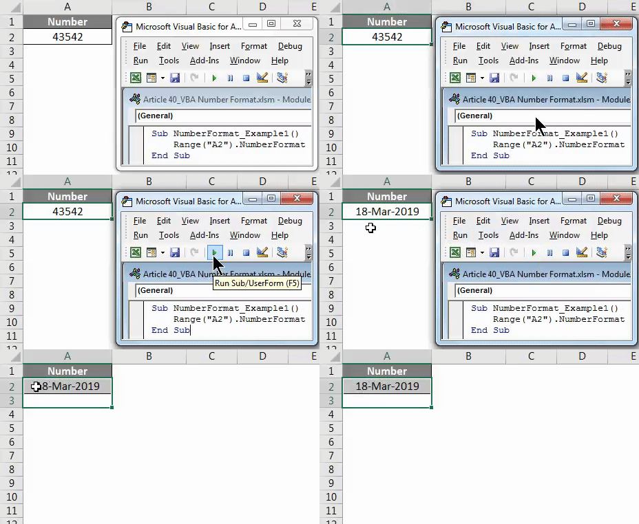
For example assume you have the number 43542 in cell A2.

Now I will apply the date format of “dd-mmm-yyyy”.

And it will display the result as 18-Mar-2019.

Similarly in VBA as well we will perform the same job by using number format property.

How to Use Number Format Function in VBA?

Let’s understand how to use Number Format Function in VBA with some examples.

Example #1

Ok, we will see how to format the same cell value using VBA code. I will remove the date format I have applied to the serial number 43542 in cell A2.

Now go to VBA editor and create a macro name.

Code:

Sub NumberFormat_Example1()

End Sub

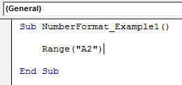
Now we need to tell which cell actually we want to format, in this case, we need to format the cell A2. So write the code as “Range (“A2”)”

Code:

Sub NumberFormat_Example1()

    Range ("A2")

End Sub

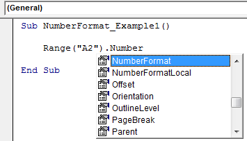
After selecting the cell to select the property called “NumberFormat” by putting dot (.)

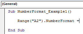
After selecting the property put an equal sign.

Now apply the format we wish to apply in this case, format is date format i.e. “dd-mmm-yyyy” format.

Code:

Sub NumberFormat_Example1()

    Range("A2").NumberFormat = "dd-mmm-yyyy"

End Sub

Now run this code, it will display the result exactly the same as the worksheet number formatting.

Example #2

Format Numbers using Built-in Formats 

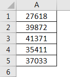
Assume you have few numbers from cell A1 to A5.

We will try out different built-in number formats. Some of the number formats are “Standard”, General”, “Currency”, “Accounting”.

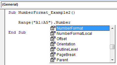
To apply the formatting we need to select the range of cells first, here the range of cells is from A1 to A5 and then select the number format property.

Apply the number format as “General”.

Code:

Sub NumberFormat_Example2()

    Range("A1:A5").NumberFormat = "General"

End Sub

Example #3

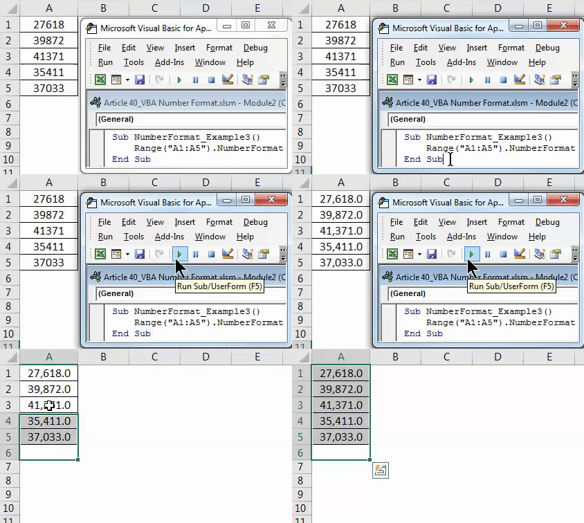
As “General” doesn’t have any impact on default numbers we don’t see changes. So apply the currency format and code for currency format is “#,##0.00”.

Code:

Sub NumberFormat_Example3()

    Range("A1:A5").NumberFormat = "#,##0.0"

End Sub

This will apply the currency format like the below.

Example #4

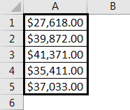
If you wish to have currency symbol you can provide the currency symbol just before the code.

Code:

Sub NumberFormat_Example4()

    Range("A1:A5").NumberFormat = "$#,##0.0"

End Sub

This code will add a currency symbol to the numbers as part of the formatting.

Example #5

Format Percentage Values

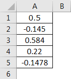
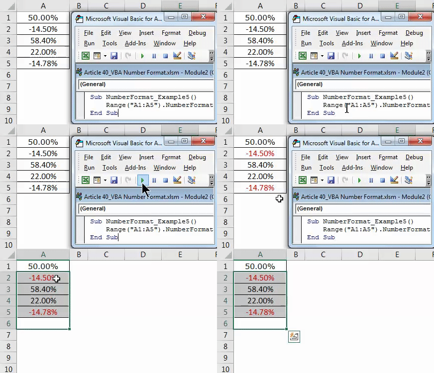
Now we will see how to format percentage values. For this example, I have created some of the percentage values from cell A1 to A5.

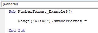
Now select the range and select Number Format property.

Apply the formatting code as “0.00%”.

Code:

Sub NumberFormat_Example5()

    Range("A1:A5").NumberFormat = "0.00%"

End Sub

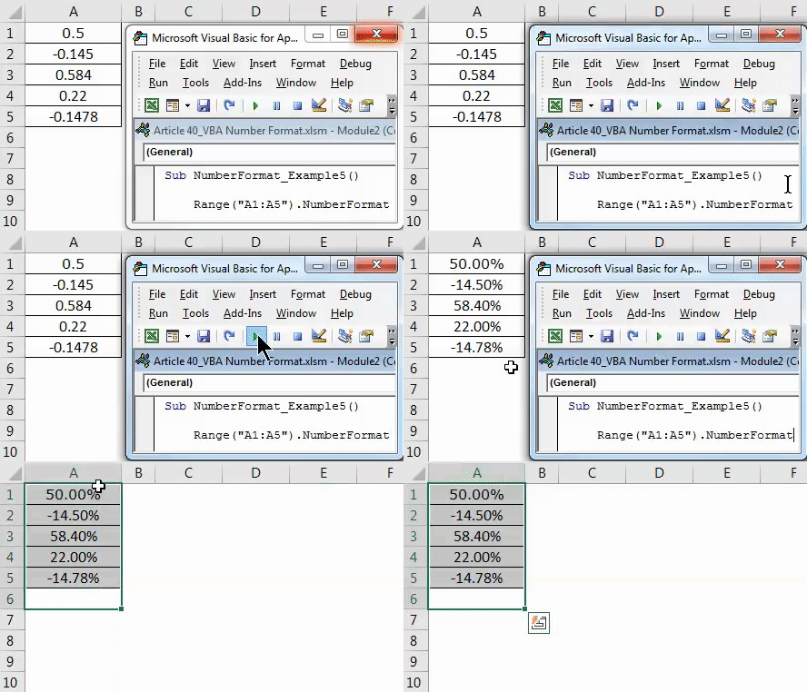
Run this code using F5 key or manually then it will convert all the values to the percentage.

Now, look at the cells a2 & a5 we have negative values. As part of the formatting, we can show the negative values in red color as well. To show all the negative values formatting code is “0.00%;[Red]-0.00%”

Code:

Sub NumberFormat_Example5()

    Range("A1:A5").NumberFormat = "0.00%;[red]-0.00%"

End Sub

Run this code using F5 key or manually and we will have all the negative percentage values in red color.

Example #6

Format Positive Numbers and Negative Numbers

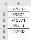
As we can format numbers we can play around with them as well. Assume few numbers from range A1 to A5 which includes negative numbers as well.

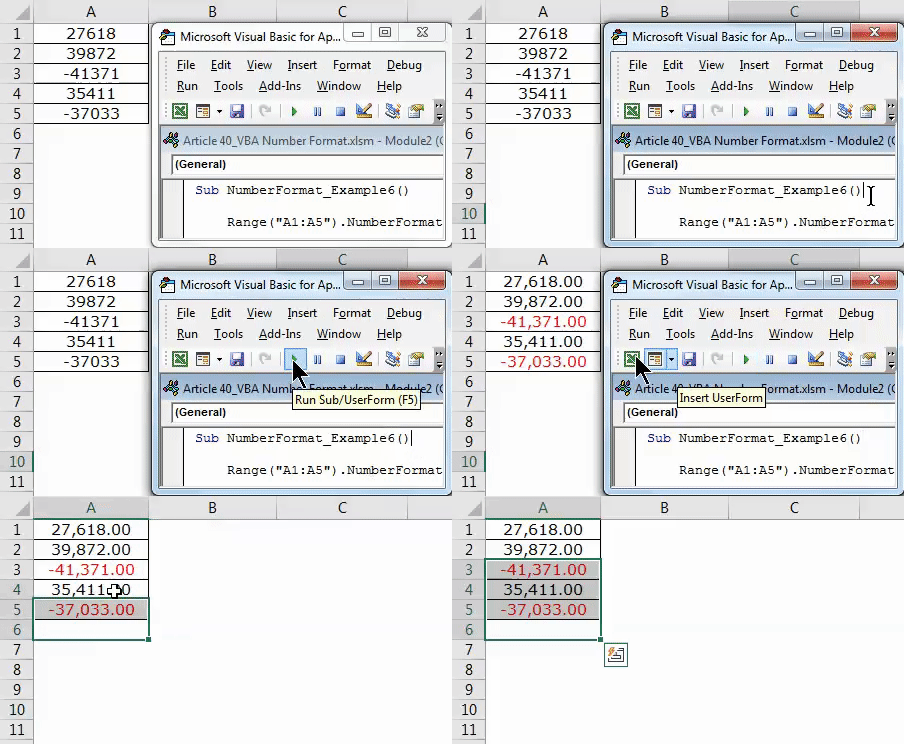
As we have shown in the percentage here also we can show all the negative numbers in red color. To show negative numbers in red color code is “#,##.00;[red]-#,##.00”

Code:

Sub NumberFormat_Example6()

    Range("A1:A5").NumberFormat = "#,##.00;[red]-#,##.00"

End Sub

This will format the numbers like this.

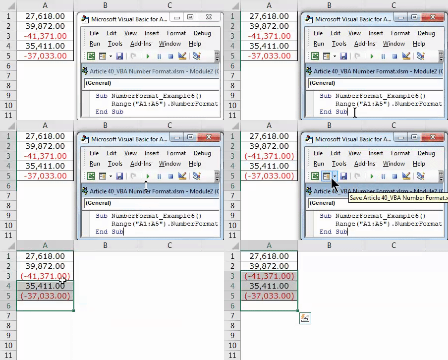
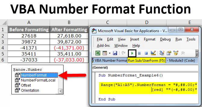
We can also show negative numbers in red as well as in brackets. To do this below is the formatting code.

Code:

Sub NumberFormat_Example6()

    Range("A1:A5").NumberFormat = "#,##.00;[red](-#,##.00)"

End Sub

Run this code using F5 keys or manually and this will format the numbers like this.

Example #7

Text with Number Formatting

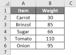
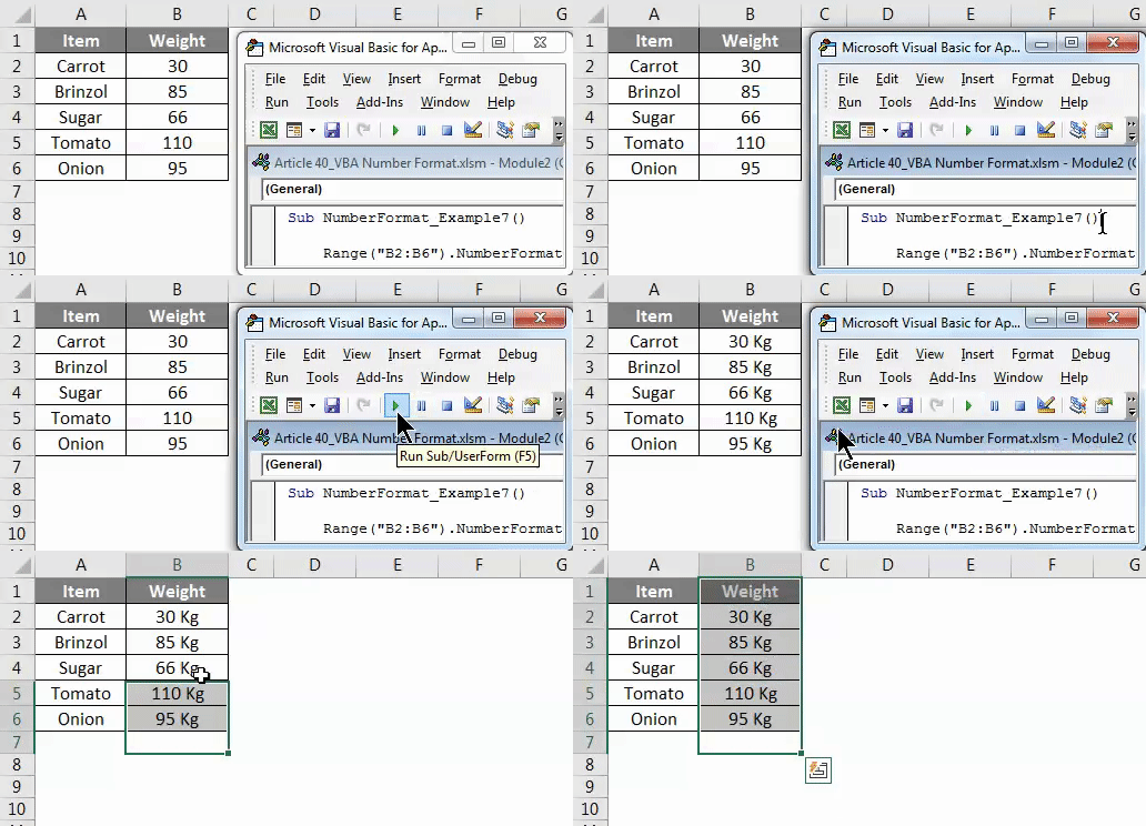
The beauty of number formatting is we can also add text values to it. I have a list of items that measure their weight in “Kg’s”.

The problem here is Carrot’s weight says 30, by looking at this weight reader cannot understand whether it is 30 grams or 30 kgs. So we will format this by using VBA code.

Code:

Sub NumberFormat_Example7()

    Range("B2:B6").NumberFormat = "0#"" Kg"""

End Sub

Run this code using F5 key or manually and this will add the word “Kg” in front of all the number from B2 to B6.

Recommended Articles

This has been a guide to VBA Number Format Function. Here we discussed how to use Excel VBA Number Format Function along with some practical examples and downloadable excel template. You can also go through our other suggested articles –

1. FIND Function in Excel with Examples
2. What is VBA Function in Excel?
3. Guide to VBA Range Object
4. How to use VBA VLOOKUP Function?
5. How to Use Negative Numbers in Excel?