VBA Range Cells

Updated June 9, 2023

VBA Range Cells

In VBA, the range is also called the property of an individual cell or a group of cells in any row or a column. The range is particularly a data set in Excel. For example, cell A1 to cell B3 is a range of cells if they contain a value of some sort or they are empty.

In VBA, we make codes to automate our tasks. To automate our tasks, we refer to the value in Excel cells. Those sets of individual or multiple cells are called range in Excel. We can specify which rows or column range we refer to in VBA.

Syntax of Range in Excel VBA

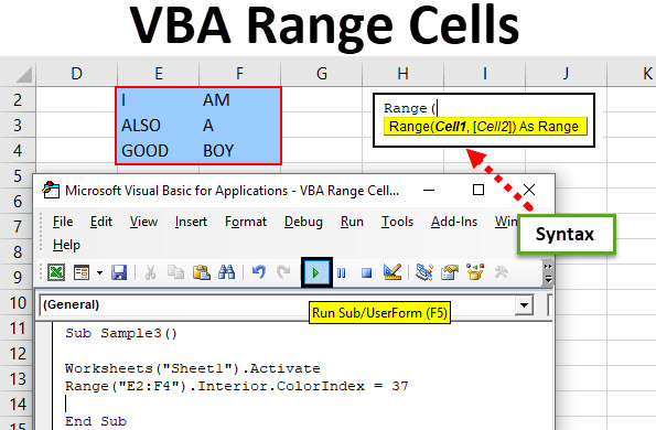
VBA Range has the following syntax:

The syntax to use range expression in VBA is as follows:

Expression.Range(“Cell Range”)

To use the range function, we need to understand three basic things in VBA –

• Object Qualifier: This is the workbook or the worksheet we refer to.
• Property: This is the function to use the properties of the object.
• Method: This function is what we want to do with the data we selected.

For example, Application.Workbooks(“ANAND.xlsm”).Worksheets(“Sheet1”).Range(“A1”) The object qualifier is Application. Workbooks in which we referred to ANAND named Excel file and Sheet 1 as a worksheet; if we have to change the font, that would be our method. This will be clear with more examples.

Let us first change the font of our cell A2, which is the Value of “ANAND,” to bold using the VBA range function.

Follow the below steps to use VBA Range Function.

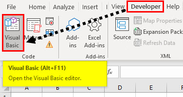
Step 1: In the developer’s tab, click on Visual Basic to open VB Editor.

Step 2: Click on Insert Tab and go to the module to open the code window.

Step 3: Declare a sub-function in the code window. Cell A2 has in sheet 1.

Code:

Sub Sample()

End Sub

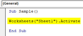
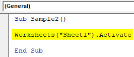
Step 4: In the code, activate the worksheet by the following code.

Code:

Sub Sample()

Worksheets("Sheet1").Activate

End Sub

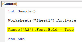
Step 5: Now, we will change the font for the specific cell using the range function in VBA.

Code:

Sub Sample()

Worksheets("Sheet1").Activate

Range("A2").Font.Bold = True

End Sub

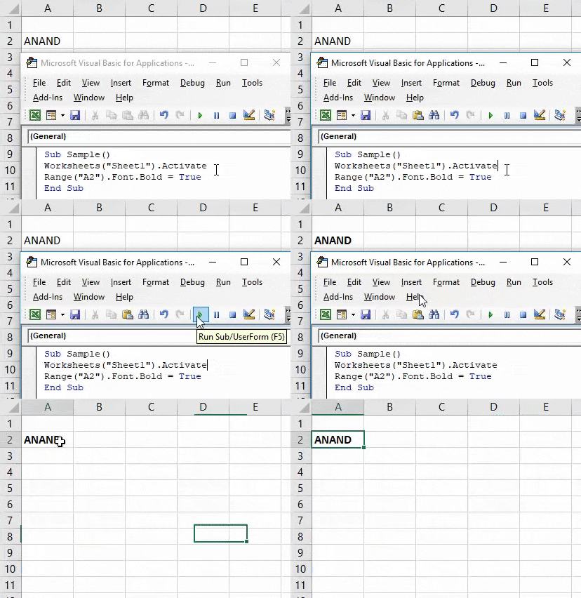
Step 6: Run the above code from the run button provided or press f5.

Once we have run the code, we can see the following result.

VBA Range Cells – Example #2

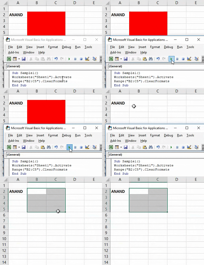
Now let us change the colors of the specific range of cells. For demonstration purposes, I have made cell range B2:C5 in red color. With the VBA range function, I want to select them and clear the font. Here is the original representation of those cells.

Follow the below steps to use Excel VBA Range Cells.

Step 1: In the developer’s tab, click on Visual Basic to open VB Editor.

Step 2: Click on Insert Tab to insert a new module to open the code window. Click on the module inserted to start writing the code.

Step 3: Declare a sub-function in the code window.

Code:

Sub Sample1()

End Sub

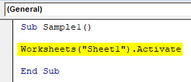
Step 4: Activate the worksheet with the below function.

Code:

Sub Sample1()

Worksheets("Sheet1").Activate

End Sub

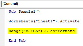
Step 5: Now, we select the cells and clear the format using the range function.

Code:

Sub Sample1()

Worksheets("Sheet1").Activate

Range("B2:C5").ClearFormats

End Sub

Step 6: Run the code, and see the result from the run button provided.

VBA Range Cells – Example #3

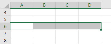
Let us merge a few cells using the VBA range function. For demonstration purposes, Let us see what the current cells look like without merging.

Follow the below steps to use Excel VBA Range Cells.

Step 1: In the developer’s tab, click on Visual Basic to open VB Editor.

Step 2: Click on Insert Tab to insert a new module to open the code window. Click on the module inserted to start writing the code.

Step 3: Declare a sub-function in the code window.

Code:

Sub Sample2()

End Sub

Step 4: Activate the workbook with the below function.

Code:

Sub Sample2()

Worksheets("Sheet1").Activate

End Sub

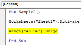
Step 5: Now, we use the VBA Range function for the merge cells as follows.

Code:

Sub Sample2()

Worksheets("Sheet1").Activate

Range("A6:D6").Merge

End Sub

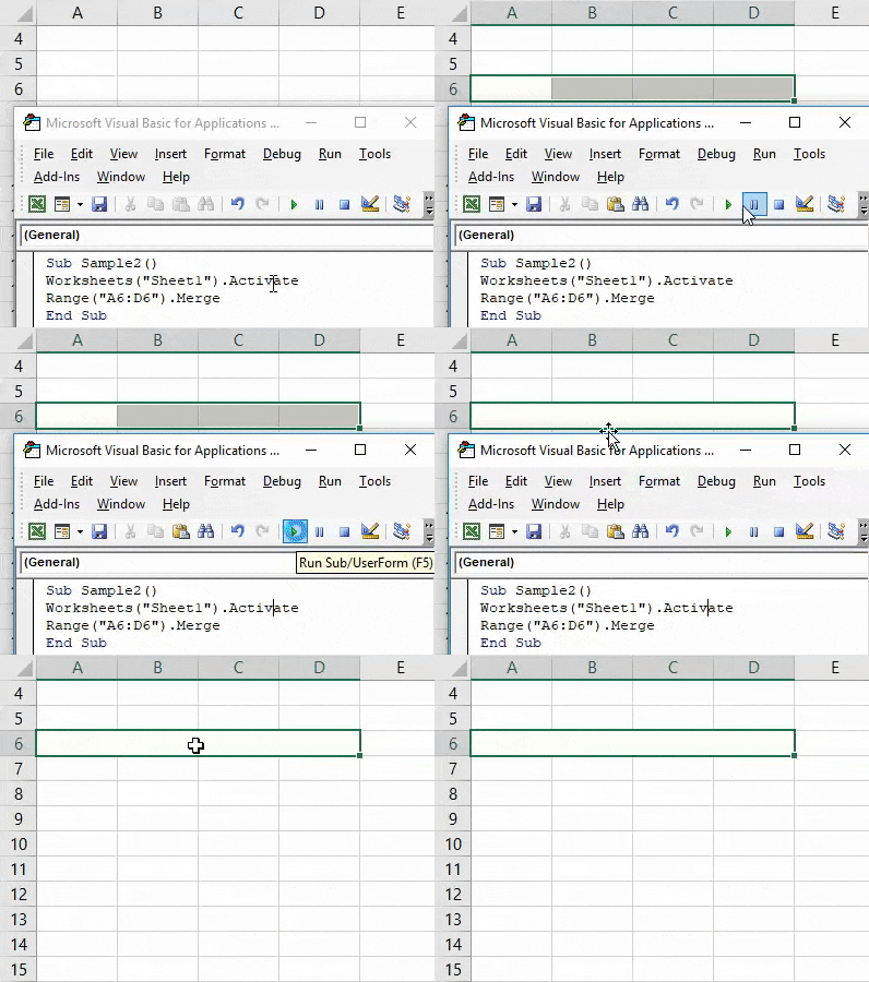
Step 6: Run the code by the run button or press f5 to see the result.

VBA Range Cells – Example #4

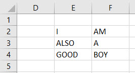
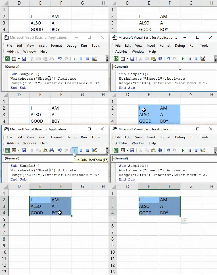
Now let us select a range of cells and change their color format. In example one, we selected only one cell. But in this example, we will select a bunch of cells of blue color. For demonstration purposes, I have data in cell range E2:F4 as follows:

Follow the below steps to use VBA Range Cells.

Step 1: In the developer’s tab, click on Visual Basic to open VB Editor.

Step 2: Click on Insert Tab to insert a new module to open the code window. Click on the module inserted to start writing the code.

Step 3: Declare a sub-function in the code window.

Code:

Sub Sample3()

End Sub

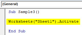
Step 4: Activate the worksheet with the following code below,

Code:

Sub Sample3()

Worksheets("Sheet1").Activate

End Sub

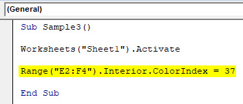
Step 5: Now, let us change the color of cell range E2:F4 using the VBA range function.

Code:

Sub Sample3()

Worksheets("Sheet1").Activate

Range("E2:F4").Interior.ColorIndex = 37

End Sub

Step 6: Run the code by pressing F5 or from the run button provided and see the result.

Things to Remember

• The range can be one cell or multiple cells.
• If we are referring to any object, we use the dot operator(.), such as range(“A1”). Select is used to select cell A1.
• We need methods and properties of a cell to use range values in Excel VBA.

Recommended Articles

This has been a guide to VBA Range Cells. Here we have discussed how to use Excel VBA Range Cells, practical examples, and a downloadable Excel template. You can also go through our other suggested articles –

1. VBA Replace
2. Excel Named Range
3. VBA Number Format
4. VBA IsError