Updated May 16, 2023
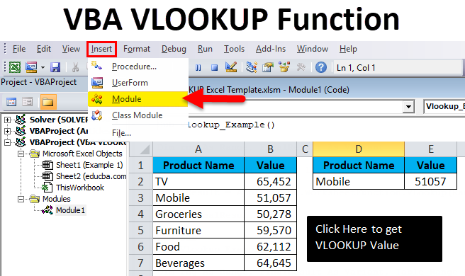
VBA VLOOKUP Function (Table of Contents)
What is VBA VLOOKUP Function?
The vlookup function of Excel can also be used in the VBA with the same syntax that we used in Excel. Open a module in VBA and define a variable for Lookup value and then declare the cell where we will be applying Vlookup using VBA. As per syntax of Vlookup in VBA, select the lookup value, lookup range or table, Column index number, and range lookup is TRUE or FALSE. If we run the code, we can see the lookup value in a declared cell in Excel.
The Formula of the VLOOKUP Function
The Formula includes four mandatory arguments.

- Lookup Value: This is the base value you are searching for. Based on this, we look for a value in the table.
- Table Value: This is the table that holds all the values. We will fetch the data from this table using the lookup value.
- Column Index Number: This is the column number we are looking for from the table. In a table, there are many columns; out of many columns, we only require the column in which we are looking for the data.
- Range Lookup: Here, we need to specify what kind of result we want. If we want the exact match, we need to mention it as FALSE or 0; if we want the approximate match, we can mention it as TRUE or 1.
Where to Write Macros?
VBA is accommodated under the Developer tab in Excel. If you cannot find the developer tab, follow the steps below to unhide this.
Step 1: Click on File.
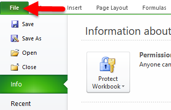
Step 2: Under File, click on Options.

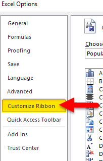
Step 3: Select Customize Ribbon.
Step 4: On the right-hand side, make sure the checkbox of the Developer tab is ticked.
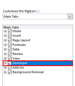
Now you must see the Developer tab in the Ribbon.

How to Use VBA VLOOKUP Function in Excel?
VBA VLOOKUP Function is very simple to use. Let us now see how to use the VBA VLOOKUP function in Excel with the help of some examples.
Example #1
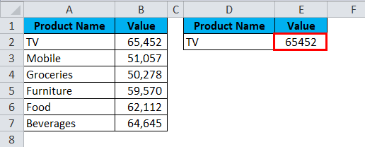
I have a sales table for different products. It has the product name and sales made against that product.
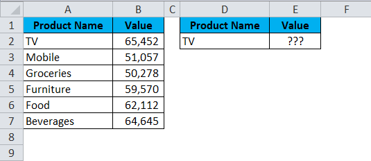
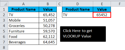
In cell E2, I want to know the sales value of the TV using the VBA VLOOKUP function.
Step 1: Go to the Developer tab and click on Visual Basic
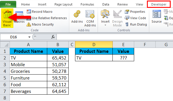
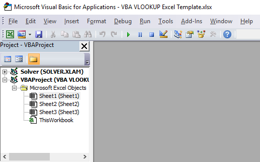
Step 2: Once you click on Visual Basic, it will open the below window for you
Step 3: Click on Insert and select Module
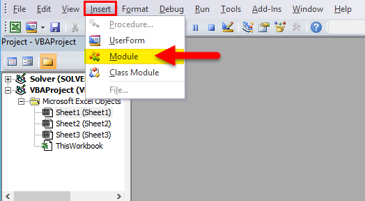
Step 4: Once you click on Module, it will insert the new Module for you. Double-click on that newly inserted Module to write your VLOOKUP code.
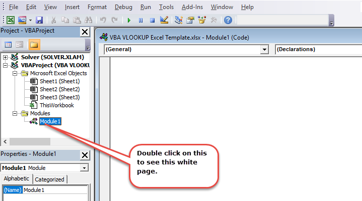
Step 5: Copy and paste the below code to your newly inserted Module.
Sub Vlookup_Example()

Dim rng As Range, FinalResult As Variant

Set rng = Sheets("Example 1").Range("E2")

FinalResult = Application. WorksheetFunction. VLookup(Range("D2"), Range("A2:B7"), 2, False)

rng = FinalResult

End Sub
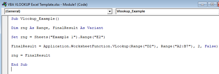
Let me break down the code to explain it to you.
Line 1: Dim rng as Range, FinalResult as Variant
This is the first line of the code. Using the DIM statement, I have declared two variables one is rng & another one is FinalResult.
Rng holds Range as the variable, and FinalResult has Variant as the variable.
Line 2: Set rng = Sheets(“Example 1”).Range(“E2”)
The previous declared variable, rng, is an object variable, so we need to set to which Range we are referring. I have set the Range to E2 cell. This is actually where I need the result to be displayed.
Line 3: FinalResult = Application. WorksheetFunction.VLookup (Range(“D2”), Range (“A2:B7”), 2, False)
This is the critical line of the code. FinalResult holds the variable of the Variant, i.e., any data type. FinalResugetsget the data from the function VLOOKUP.
Line 4: rng = FinalResult
The initial variable rng is equal to the value of FinalResult. Rng means E2 cell, and FinalResult means the value returned by the VLOOKUP function.
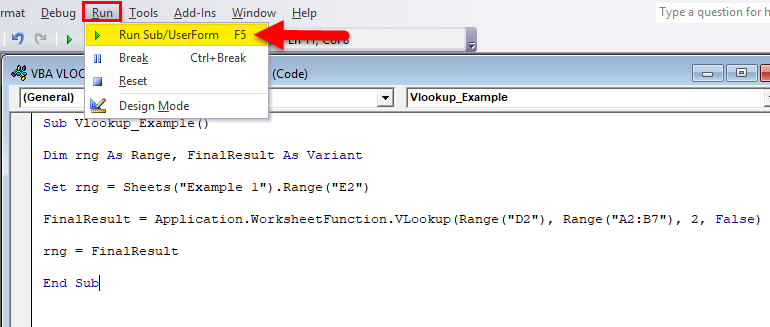
Step 6: Hit the RUN button or Press F5 to execute the code
Step 7: We will get the below output.
Example #2
Take the same data from the above example. Here I will create names and apply the same in the VLOOKUP. The code will be the same as the previous example. Only in VLOOKUP I am changing references.
Sub Vlookup_Example1()

Dim rng As Range, FinalResult As Variant, Table_Range As Range, LookupValue As Range

Set rng = Sheets("Example 1").Range("E2")

Set Table_Range = Sheets("Example 1").Range("A2:B7")

Set LookupValue = Sheets("Example 1").Range("D2")

FinalResult = Application. WorksheetFunction. VLookup(LookupValue, Table_Range, 2, False)

rng = FinalResult

End Sub
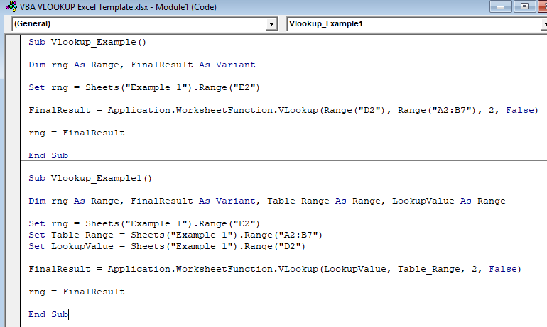
The lookup value is set to D2 cell in the name of LookupValue. Table Array is set to A2 to B7 in the name of Table_Range.
Create a Macro Button
Once the macro code is written, we need to design the macro.
Step 1: Go to Insert and Select the rectangular shape.
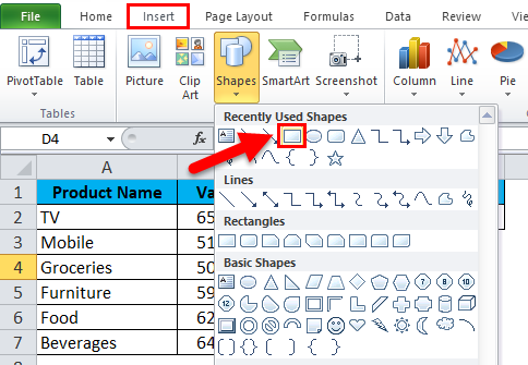
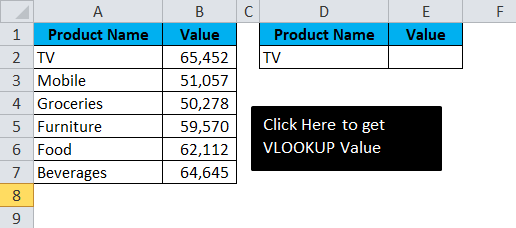
Step 2: Draw a rectangular shape
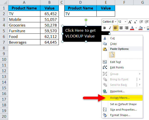
Step 3: Once the Rectangular shape has been drawn right, click on the rectangular shape and click on Assign Macro.
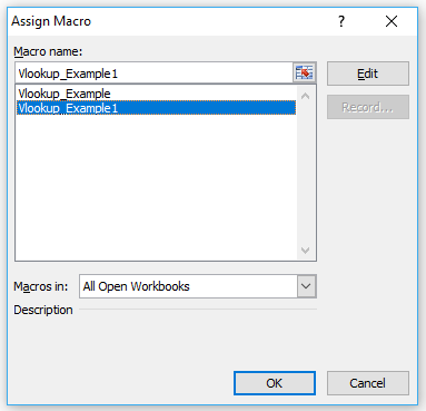
Step 4: Once you click on Assign Macro, it will open up all the macro names. Select the macro name you wish to assign. I am assigning the Example 1 macro name to the rectangular shape.
Step 5: Now rectangular shape has become a macro button. You will get the output below once you click on the rectangular shape.
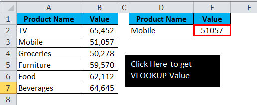
You can change the lookup value to cell D2 and get the result. I have changed the D2 cell value to Mobile in the image below.
Things to Remember About VBA VLOOKUP
- In VBA too VLOOKUP works the same as the worksheet function.
- Declaring variables and assigning data types is the important thing here.
- In the resulting cell, we do not see any formula. Any value returned by the VBA function does not hold any formula.
Recommended Articles
This is a guide to the Excel VBA VLOOKUP function. Here we discuss the VLOOKUP Formula and how to use VBA VLOOKUP in Excel, with practical examples and a downloadable Excel template. You can also go through our other suggested articles –

