Table of Contents
Introduction to VLOOKUP For Text in Excel
While using VLOOKUP in Excel to find any particular value, it is necessary that the format of the data in both the lookup table and the lookup value is the same. Mostly, we use VLOOKUP in Excel to search only numerical data, but if you are using both text and number formats, you can get an #N/A error.
It happens when the lookup value and the data table have different formats, i.e., one is in number, and the other is in text. Here, VLOOKUP shows a #N/A error because it cannot find a match. So, when we use it to find text-based values, you can use VLOOKUP for text to fix the error.
Before we learn the methods to solve this error, let us first understand how this error occurs with the help of an example.
Example: #N/A Error due to Numbers Stored as Text
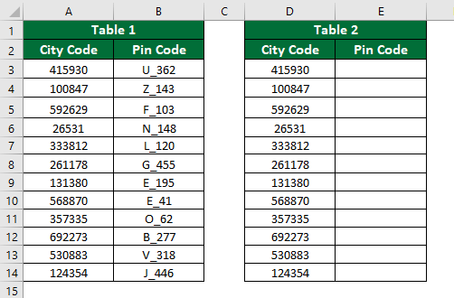
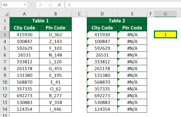
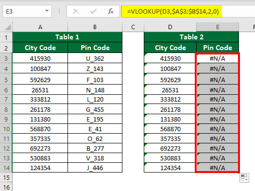
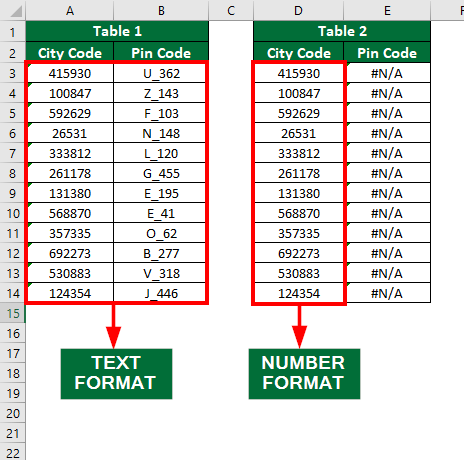
Here, we have two tables. Table 1 is the main table with city codes, and their specific pin codes, and Table 2 is our lookup array. Let us try to find the pin code for the city code “415930”.
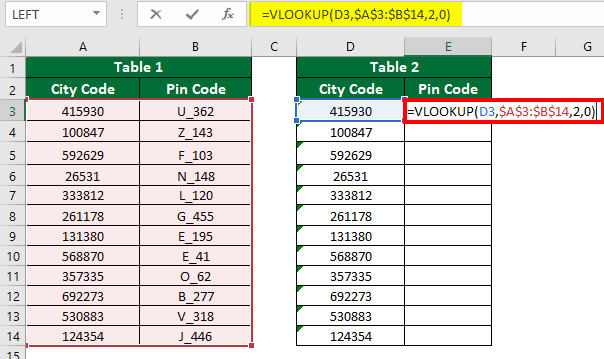
- Enter the following VLOOKUP formula in cell E3.
- Press Enter and then drag the formula until E14.
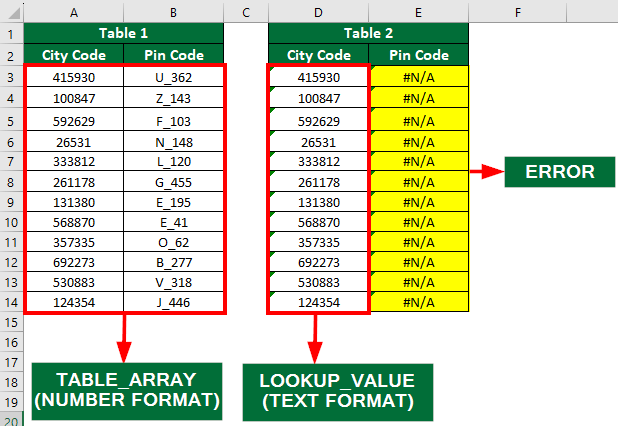
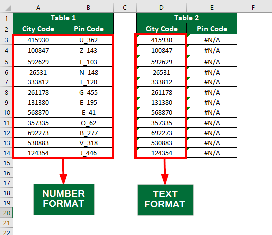
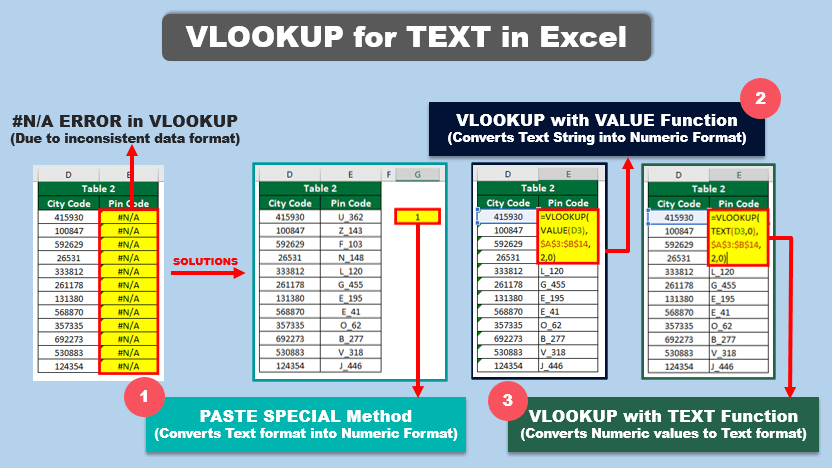
When we use the VLOOKUP Function in Column E, it shows a “#N/A” error. It happens because the lookup_value (Column D) is in text format, and the table_array (Columns A & B) is in numeric format.
Therefore, to avoid this error, make sure the lookup value and the table values are in the same format.
How to Use VLOOKUP for Text?
To solve this #N/A error, we must make sure that the data table and lookup values are in the same format, i.e., either in text or number format. The Excel functions to correct this error are as follows:
- Paste Special feature
- VALUE function
- TEXT function (for reverse conversion)
Example #1 – Convert Text to Numeric Values Using the Paste Special Method
The values in Column D look like numbers but are in text format. In this example, we will convert values in column D to number format by using the Paste Special method.
Solution:
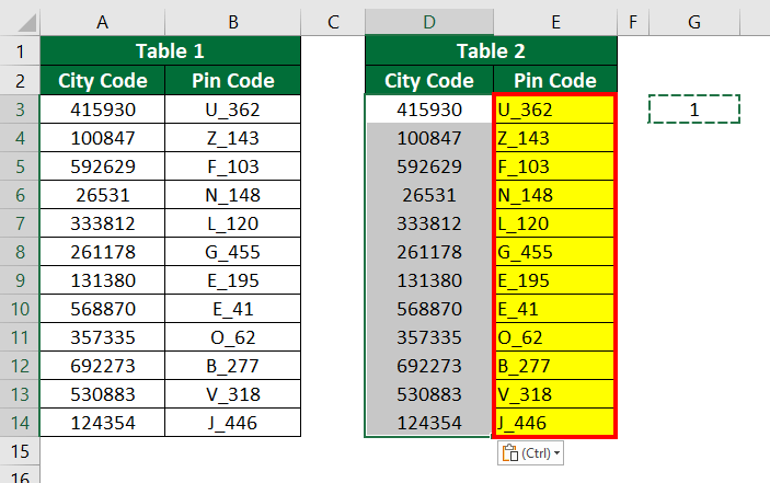
Step 1: Select “Cell G3” and enter number 1.
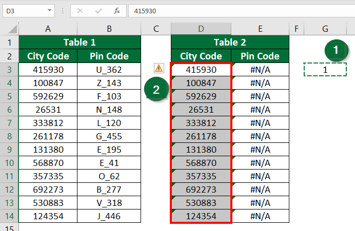
Step 2: Copy “Cell G3” and select the range from Cell “D3 to D14”, as shown below.
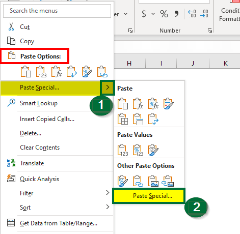
Step 3: Right-click the selected range and select the “Paste Special” option, as shown below. You can also use the keyboard shortcut “Ctrl +Alt +V” to open the “Paste Special” window.
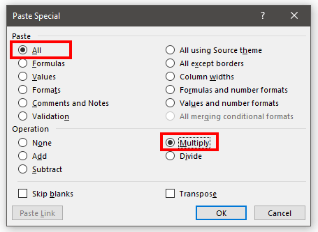
Step 4: Select the “All” option under “Paste” and “Multiply” under the “Operation” section.
Step 5: Click on the OK button.
The format of Column D will change from text to number after applying the “Paste Special” method. Therefore, the VLOOKUP Function will give the correct match instead of the #N/A error.
Example #2 – Convert Text to Numeric Values Using the VALUE Function
We use the VALUE() function within the VLOOKUP function to directly change the format of a text-based cell into a numeric value.
Let us take the same data as Example #1.
Solution:
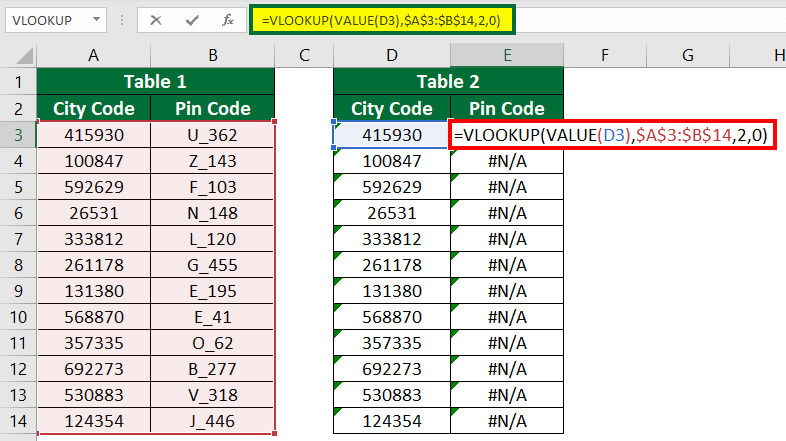
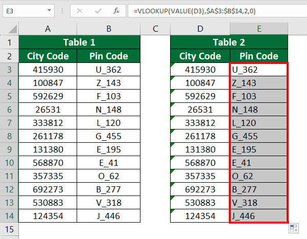
Step 1: Select “Cell E3” and add the VALUE Function within the VLOOKUP function as follows:
Step 2: Press “Enter”.
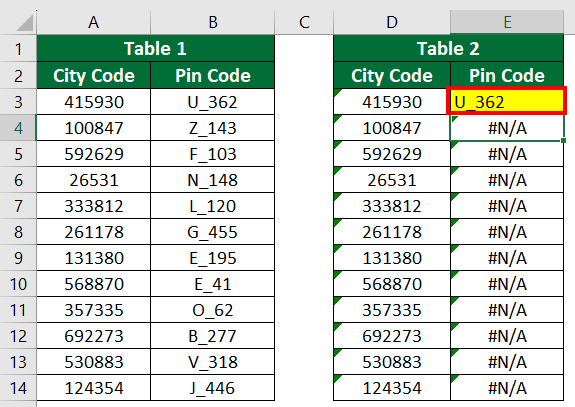
The formula will display “U_362” in Cell E3.
Step 3: Drag the cell downwards to copy the formula in cell E3 to E14.
The formula will now display the actual pincode instead of a #N/A error.
The VALUE function changed the text form of lookup_value (Column D) into the numeric form so that the VLOOKUP function could fetch accurate results.
Example #3 – Convert Numeric to Text Values Using the TEXT Function
In all the above examples, the lookup_value (Column D) was in text format, and the table_array (Columns A & B) was in a numeric format. Hence, we changed the format for the lookup_value (Column D) from text to number.
Now, let us see how to change the data format from numeric to text format.
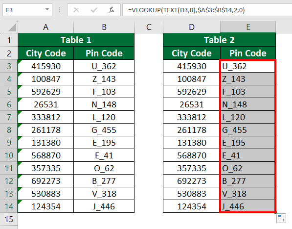
Consider the same data from the above example. But this time, your original data, i.e., Column A, is in text format, and the lookup_value (Column D) is in numeric format. So, we have to use the TEXT function to convert the lookup_value from the number format into text format.
Solution:
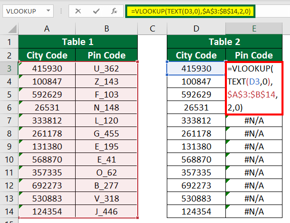
Let us change the data formatting by simply adding the TEXT Function.
Step 1: Select “Cell E3” and enter the formula:
Step 2: Press “Enter”.
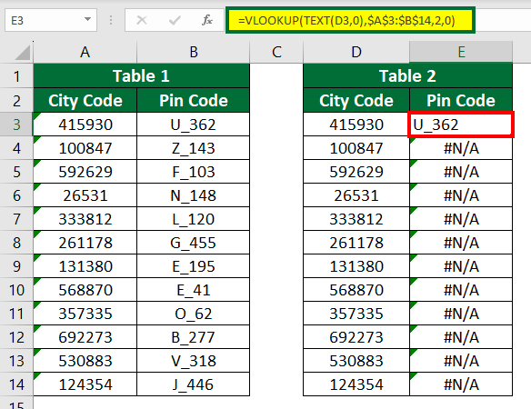
The formula displays “U_362” in “Cell E3”.
Step 3: Drag “Cell E3” downwards. The formula will display the accurate result throughout Column E.
Here, the TEXT function has first changed the lookup_value (D3) number format into text format.
Frequently Asked Questions (FAQs)
Q1. Does VLOOKUP work with alphanumeric data?
Answer: Yes, VLOOKUP can handle alphanumeric data in Excel. It’s a function that finds a specific value from a huge data table. It doesn’t matter if the values are a mix of letters and numbers. Just make sure the data formatting is consistent.
Q2. Why won’t VLOOKUP work with text?
Answer: VLOOKUP for text can give an error in the following situations:
- If data is present in both text and number format.
- When the value you are looking for does not match the values in the original data.
- If there are spelling mistakes or the data is in the wrong order.
- If the table is not in ascending order before applying the function.
- If there are extra spaces in the original data or lookup data.
Recommended Articles
This EDUCBA article explains how to use VLOOKUP for text using various Excel functions. Here, we have mentioned methods that you can use to solve the #N/A error using practical examples and an Excel template. Read the following articles to learn more.
