Updated March 24, 2023

Introduction to Weak Law of Large Numbers
The Law of Large Numbers is an important concept in statistics that illustrates the result when the same experiment is performed in a large number of times. As per the theorem, the average of the results obtained from conducting experiments a large number of times should be near to the Expected value (Population Mean) and will converge more towards the expected value as the number of trials increases. There are two different versions of the Law of Large numbers which are Strong Law of Large Numbers and Weak Law of Large Numbers, both have very minute differences among them. Weak Law of Large Number also termed as “Khinchin’s Law” states that for a sample of an identically distributed random variable, with an increase in sample size, the sample means converge towards the population mean.
For sufficiently large sample size, there is a very high probability that the average of sample observation will be close to that of the population mean (Within the Margin) so the difference between the two will tend towards zero or probability of getting a positive number ε when we subtract sample mean from the population mean is almost zero when the size of the observation is large.
Definition of Weak Law of Large Numbers
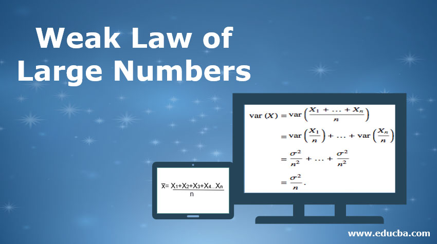
For Independent and identically distributed random variables X1, X2, Xn the sample mean, denoted by x̅ which is defined as,
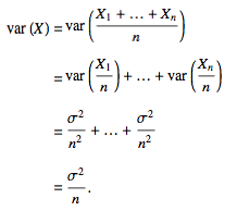
In addition,
By using the Chebyshev inequality,
As per Bernoulli’s Theorem,
Where x̅ is the sample mean for sufficiently large sample size and μ is the population mean.
Interpretation: As per Weak Law of large numbers for any value of non-zero margins, when the sample size is sufficiently large, there is a very high chance that the average of observation will be nearly equal to the expected value within the margins. The weak law in addition to independent and identically distributed random variables also applies to other cases. For example, if the variance is different for each random variable but the expected value remains constant then also the rule applies. If the variance is bounded then also the rule applies as proved by Chebyshev in 1867. Chebyshev’s proof works as long as the variance of the first n average value converges to zero as n move towards infinity.
Example: Consider a fair six-sided dice numbered 1, 2, 3, 4, 5 and 6 with equal probability of getting any sides. So the expected value from any roll is,
(1+2+3+4+5+6)/6 =3.5
So, as per the law of large numbers, when you roll dices a large number of times, the average of their value approaches closer to 3.5, the precision increases even further as the number of trials increases. Another example is the Coin Toss. The theoretical probability of getting ahead or a tail is 0.5. As per the law of large numbers, as the number of coin tosses tends to infinity the proportions of head and tail approaches 0.5. Intuitively, the absolute difference between the number of heads and tails becomes very low when the number of trails becomes very large.
Applications of Law of Large Numbers
Here are the applications of law of large number which are explained below:
1. Casino’s Profit
A Casino may lose money for small number of trials but its earning will move towards the predictable percentage as number of trials increases, so over a longer period of time, the odds are always in favor of the house, irrespective of the Gambler’s luck over a short period of time as the law of large numbers apply only when number of observations is large.
2. Monte Carlo Problem
Monte Carlo Problems is based on the law of large numbers and it is a type of computational problem algorithm that relies on random sampling to get a numerical result. The main concept of Monte Carlo Problem is to use randomness to solve a problem that appears deterministic in nature. They are often used in computational problems which are otherwise difficult to solve using other techniques. Monte Carlo methods are mainly used in three categories of problem namely: Optimization problem, Integration of numerals and draws generation from a probability distribution.
Limitations of Law of Large Numbers
In some cases, the average of a large number of trials may not converge towards the expected value. This happens especially in the case of Cauchy Distribution or Pareto Distribution (α<1) as they have long tails. Cauchy Distribution doesn’t have expectation value while as for Cauchy Distribution the expectation value is infinite for α<1. These distributions don’t converge towards the expected value as n approaches infinity.
Difference Between Strong Law of Large Numbers and Weak Law of Large Numbers
The difference between weak and strong laws of large numbers is very subtle and theoretical. The Weak law of large numbers suggests that it is a probability that the sample average will converge towards the expected value whereas Strong law of large numbers indicates almost sure convergence. Weak law has a probability near to 1 whereas Strong law has a probability equal to 1. As per Weak law, for large values of n, the average is most likely near is likely near μ. Thus there is a possibility that ( – μ)> ɛ happens a large number of times albeit at infrequent intervals. With Strong Law, it is almost certain that ( – μ)> ɛ will not occur i.e the probability is 1.
Conclusion
The law of large numbers is among the most important theorem in statistics. The law of large numbers not only helps us find the expectation of the unknown distribution from a sequence but also helps us in proving the fundamental laws of probability. There are two main versions of the law of large numbers- Weak Law and Strong Law, with both being very similar to each other varying only on its relative strength.
Recommended Articles
This is a guide to the Weak Law of Large Numbers. Here we discuss the definition, applications, distinction and limitations of the weak law of large numbers. You can also go through our other suggested articles to learn more –


