Excel Wildcard (Table of Contents)
Introduction to Wildcard in Excel
The wildcard characters in Excel are the most underrated feature of Excel, and most people don’t know about it. It is a very good to know feature as it can save a lot of time and effort required to do some research in Excel. We will learn about Excel wildcard characters in detail in this article.
There are 3 Wildcard Characters in Excel:
- Asterisk (*)
- Question Mark (?)
- Tilde (~)
These three wildcard characters have a different purposes from each other.
1. Asterisk (*) – The Asterisk represents any number of characters in the text string.
For Example, when you type Br*, it could mean Break, Broke, or Broken. So * after Br could mean to select only words which start with Break. It doesn’t matter what words or number of characters are thereafter Br. You can similarly start the search with Asterisk.
For Example, *ing it could mean Starting, Ending, or Beginning. So * before ing could mean to select only words that end with ‘ing’, and it doesn’t matter what words or the number of characters are there before ing.
2. Question Mark (?) – The Question marks are used for a single character.
For Example,?ove could mean Dove or Move. So here, the question mark represents a single character, M or D.
3. Tilde (~) – We have already seen two wild characters, Asterisk (*) and Question Mark (?). The third wildcard character, Tilde (~), is used to identify the wildcard character. We have not encountered many situations where we need to use tilde (~), but it’s good to know the feature in Excel.
How to Use Wildcard Characters in Excel?
Let’s now look at the below examples to use wildcard characters in Excel.
Example #1 – Filtering Data with Wildcard Characters
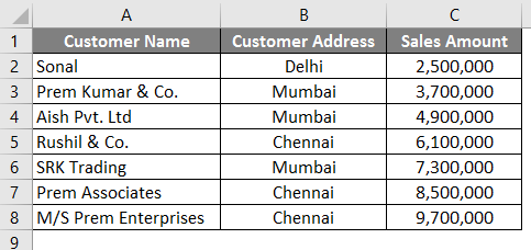
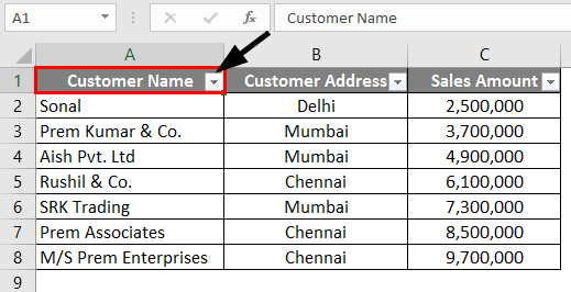
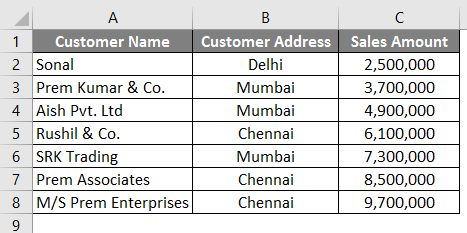
Suppose you are working on the sales data where you have the customer name, address, and sales amount, as given in the screenshot below. In the customer list, you have different companies of the parent company, “prem enterprise”. So if I need to filter all the companies of Prem in the customer name, I will just filter with one Asterisk behind Prem and one Asterisk after Prem, which will look like “*Prem*” and the search option will give me the list of all companies which has Prem in the company name.
Follow the steps below to search and filter the companies with “Prem” in their name.
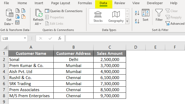
- Go to the Data tab in Excel.
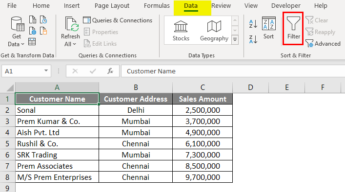
- Click on the Filter option.
- Once the filter is applied, go to column A, “Customer Name”, and click on the drop-down box.
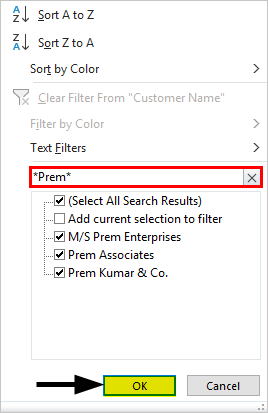
- Type “*Prem*” in the search field and click OK.
- As you can see, all three companies which have “Prem” in their name have been filtered and selected.
Example #2 – Find and Replace Using Wildcard Character
The area where we can use the wildcard characters effectively to find and replace words in Excel. Let us take a similar example of what we used in Example 1.
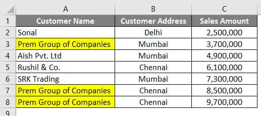
In the first example, we filtered the companies’ names with “Prem” in them. So in this example, we will try to find the companies that have “prem” in their name and replace the name of the company with the name “Prem Group of Companies”. So to do this, you need to follow the below steps.
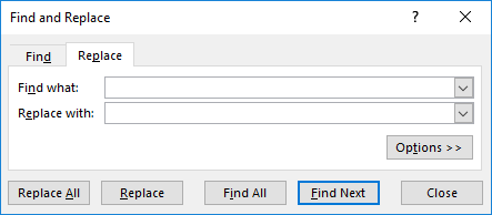
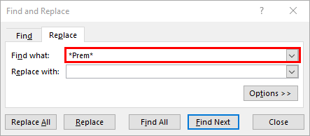
- Press CTRL + H in Excel, and you will see the below screen open.
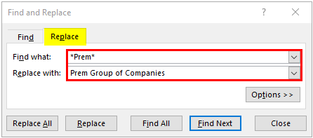
- In the Find what field, enter the word “*Prem*” to search the name of the companies with “Prem” in its name.
- Enter “Prem Group of Companies” in the Replace with the option.
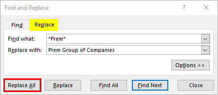
- Now click on the “Replace All” button so that it will replace all the name of the companies which has “prem” in their name with “Prem Group of Companies”.
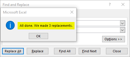
- After clicking the “Replace All” button, we will get the dialog box below.
You can see that the companies’ name in row 3, 7 & 8 is changed to “Prem Group of Companies”.
Example #3 – Vlookup Using Wildcard Character
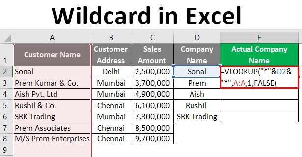
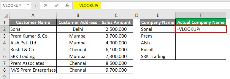
Like we used to find and replace with the help of wildcard characters, we can also use wildcard characters in Excel Vlookup. We will take a similar example of example 1. But in addition to the data in example 1, we have a table with an initial reference of the company name in column E.
The normal lookup will not work here as the names are not similar in columns A & F. So we need to give a lookup so that it should pick up the result for the company names in column A.
Follow the below steps to see how we can do that.
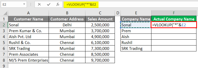
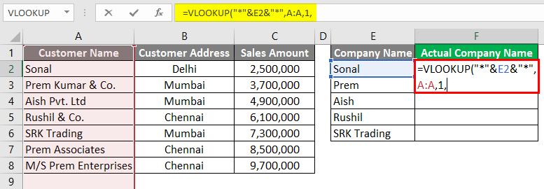
- Enter the formula for Vlookup in column F2, as shown in the below screenshot.
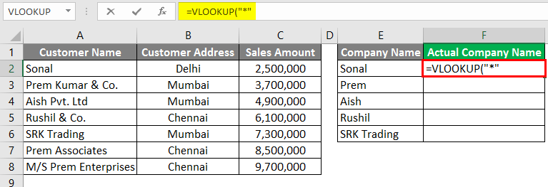
- Start the Vlookup value with an asterisk between the semicolons “*” as shown in the screenshot below.
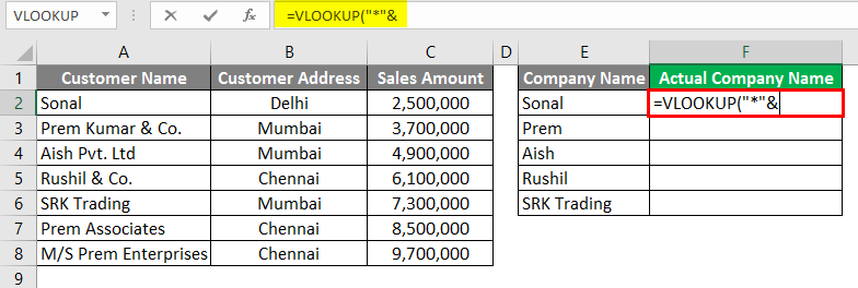
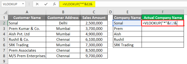
- Now type “&” to connect the reference with cell E2.
- Give the reference for cell E2.
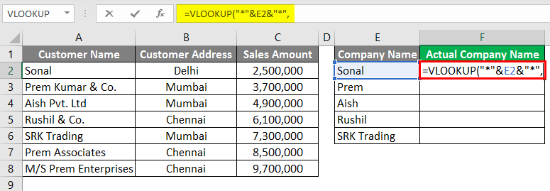
- Again type “&” after the cell reference.
- Now end the Vlookup value with an asterisk between the semicolons “*” as shown in the screenshot below.
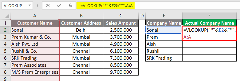
- For the Table_Array in vlookup, give column A’s reference so that it should pick up the value from Column A.
- In the column Index, you can select 1 as we need the value from column A itself.
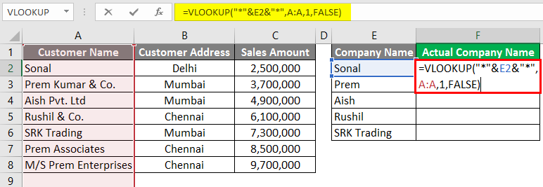
- For the last condition in the VLOOKUP formula, you can select FALSE for the Exact match.
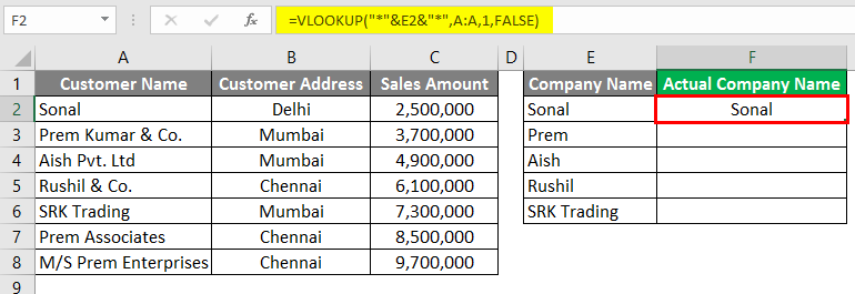
- Press Enter key.
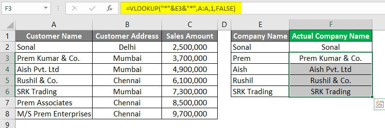
- Now you can drag down the formula to the below row and see the result.
As you can see, the lookup has picked up the value from column A, even though the names were not the same in column F.
Things to Remember About Wildcard in Excel
- The wildcard characters must be used carefully because they can result from other options that can arrive with the same logic. You may need to check on those options. For example, in example 3, where we look up with the help of wild card character, there were 3 companies with “Prem” in its name, but look captured only the first company name, which has “prem” in its name in column A.
- Wildcard characters can be used in other Excel functions like Vlookup, count, match, etc. So you can use a wildcard character in many innovative ways.
- We can also use the combo of Asterisk (*) and question mark (?) in a few situations if required.
Recommended Articles
This is a guide to Wildcard in Excel. Here we discuss How to Use Wildcard Characters in Excel, practical examples, and a downloadable Excel template. You can also go through our other suggested articles –
