Updated May 3, 2023
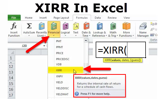
XIRR Function in Excel
XIRR function is also one of the financial functions in Excel, which is used to calculate the Internal Rate of Return (IRR) in any series of intervals. XIRR function works when we assign the dates of obtained intervals, whether regular or irregular and calculates the internal rate of return on that array of cash flow. The good thing about XIRR Function is it considers only irregular series of cash flow or installment intervals. In contrast, most of the functions in Excel give fine results when a regular interval series is selected.
Returns:
XIRR is popular in spreadsheet analysis because, unlike the XIRR function, it allows for irregular periods between compounding dates. The XIRR function is especially useful in financial structures because the timing of the initial investment within the month can have a meaningful effect on the XIRR. For instance, a large equity investment on the 1st of the month produces a much lower XIRR than the same sized equity investment on the last day of the same month. The XIRR Function provides the exact number of days in the first period by allowing for variable compounding periods. Therefore, it can help assess the effect of a delay in the partnership formation date within the same month.
XIRR Function also has a few of its unique flaws. Because it uses Excel’s internal actual date logic, using the XIRR function with even monthly periods consistent with 30/360 loan interest calculations is impossible. Also, a well-known bug with the XIRR function as of this writing is that it cannot handle a set of cash flows that start with zero as its initial value.
XIRR Formula in Excel
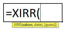
Below is the XIRR Formula.
How to Open XIRR Function?
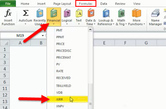
Click on Formula Tab > Financial > Click on XIRR
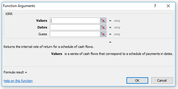
We Get A New Function Windows Showing In Below Mention Picture.
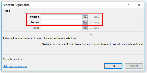
Then we have to enter the details of cash value and dates.
The shortcut of using the XIRR Formula
Click on the cell where you want the result value, then put the formula as below mentioned
= XIRR (cash flow value range, dates value range) > Enter
XIRR formula has the following arguments:
- Values (Required Argument) –The values representing the series of cash flows. Instead of an array, it can reference a range of cells containing values.
- Dates (Required Argument) – A series of dates corresponding to the given values. Subsequent dates should be later than the first date as the first date is the start date, and subsequent dates are future dates of outgoing payments or income.
- Guess (Optional Argument) –It is an initial guess of the IRR. If omitted, Excel takes the default value, which is 10%.
The format of the result
It is the internal interest rate, so we consider it in the percent (%) number format.
How to use the XIRR Function in Excel?
This XIRR function is very simple and easy to use. Let us now see how to use XIRR in Excel with the help of some examples.
Example #1
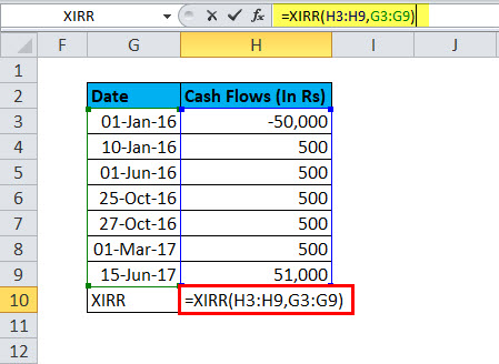
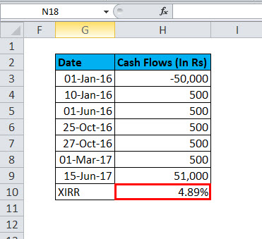
Calculating XIRR value using XIRR Formula =XIRR(H3: H9, G3: G9)
The answer will be 4.89%
In the above table, the interest inflows are irregular. Hence, you can use the XIRR function in Excel to compute
The internal rate of interest on these cash flows, the investment amount is showing a minus sign. When you get the result, then change the format with %.
Example #2
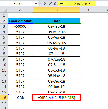
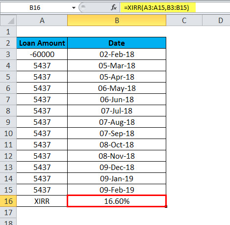
Suppose you are given a loan, details are mentioned in the below +table, loan of rupees 6000 showing a minus sign(-), and receive date is 2 Feb-18, after that rest date and the amount for EMI. Then we can use the function XIRR for the internal rate return of this amount.
Calculating XIRR value using XIRR Formula =XIRR(A3: A15, B3: B15)
The answer will be 16.60%
In an Excel sheet, first, enter the original amount invested. A ‘minus sign should represent the amount invested. In the following cells, enter the returns received during each period. “Remember to include the ‘minus’ sign whenever you invest the money.
Now, find XIRR using the values that refer to a series of cash flows corresponding to a schedule of payments in dates. The series of values must contain at least one positive and one negative value. The first payment refers to the investment made at the beginning of the investment period and must be a negative value. All succeeding payments are discounted based on a 365-day-year.
The date is when the first investment and the returns were received. Each date should correspond to its respective investment made or income received, as shown in the above table. Dates should be entered in a ‘DD-MM-YY (date-month-year)’ format, as errors can occur if the format is not followed. If any number in the dates is invalid, or the format of dates is inconsistent, XIRR will reflect the “#value!” Error.
If we discuss error problems, this is also an important part. If our data is not correct, we will face such a type of issue as below mention.
- #Num! Occurs if either:
- The supplied values and date arrays have different lengths.
- The supplied values array does not contain at least one negative and at least one positive value;
- Any of the supplied dates proceeds to the first supplied date.
- The calculation needs to converge after 100 iterations.
- #value! : – occurs if any supplied dates need to be recognized as valid Excel dates.
- If you attempt to input dates in text format, there is a risk that Excel may misinterpret them, depending on the date system or data interpretation settings on your computer.
Recommended Articles
This has been a guide to XIRR Function. Here we discuss the XIRR Formula and how to use XIRR Function along with practical examples and downloadable Excel templates. You can also go through our other suggested articles –
